
Two weeks A long time ago we saw how to optimize a fuselage’s cross-sectional area using OpenVSP as a heuristic. The point of this exercise was to see if we could design the most basic optimization algorithm. The outcome of the exercise was easy to predict; as an object’s cross-sectional area reduces, so does its drag coefficient. So we wrote a simple 1 dimensional hill climb algorithm, that decreased its stepping distance as time ran out. The results were what we expected. Now we can try to do something a bit more complex: messing with the wires that connect cross-sections of the fuselage.
The Problem
Let’s begin by seeing what we can control with OpenVSP. For each cross-section of the FuselageBase we have a Skinning tab, which allows us to modify the “mesh of wires” that connect one cross-section to another. For each cross-section we have 4 parts (top, right, left, bottom) which have properties angle, slew, strength and curvature. We’ll stick to angle, slew and strength for now, because curvature is a little to complex (and it’s disabled by default on the UI). This means we have 3 variables for each point on a segment, which can change independently on 7 different segments. Assuming we can only change one attribute for each step (for example the left slew of the 4th cross-section by 10%), we can have a total of (84 * however many points there are on a segment) potential next steps. We might be tempted to optimize one cross-section at a time (as in: start from the front and work our way back) in order to simplify our algorithm, which for other problems might be perfectly acceptable, but in this case is a trap. Let’s see a simple example to make this point: imagine our algorithm finds that setting the angle of cross-section 4 to be parallel to the y axis (as in: horizontal) is the way to go. If we then move on to cross-section 5, we will be forced to find the most aerodynamic angle based on the fact that the “wire mesh” coming from cross-section 4 is horizontal. This might not be as efficient as having cross-section 4 with an angle around -5°. If we treat every cross-section independently, we will miss out on these possibilities. Furthermore, the solution space for this case is slightly stranger than the previous problem; I honestly cannot tell if a pointy tip is better than a round tip.

This is the big difference between this problem and the last; now we cannot assume anything about the solution space, and we have a multidimensional solution space to explore, meaning we don’t only have two directions we could be headed towards (increasing or decreasing the area for the previous problem), we have 3 of them for each point on each of the 7 segments. We will need a more sophisticated algorithm. But before we get into the algorithm, let’s define our boundary conditions. There are one and a half:
-
The back of the fuselage needs to remain perpendicular to the
yaxis (as in: vertical). The reason for this is so the propeller can have enough clearance from its axis to theFuselageTail. We can easily achieve this by skipping cross-sections 1, 2 and 3 (or 0, 1, 2 in programming terms). -
The front of the fuselage has to arch just enough to leave room for the pilot’s feet. I am seriously tempted to just assume this will naturally happen, or that the seating position can be rearranged afterwards. You see, it will be a rather nasty job to find a way to tell if we’re past the boundary or not, and frankly, the seating pilot’s position is aleatory. As long as it “looks natural”, we can get by.
But before we start, let’s take a good look at the starting model:
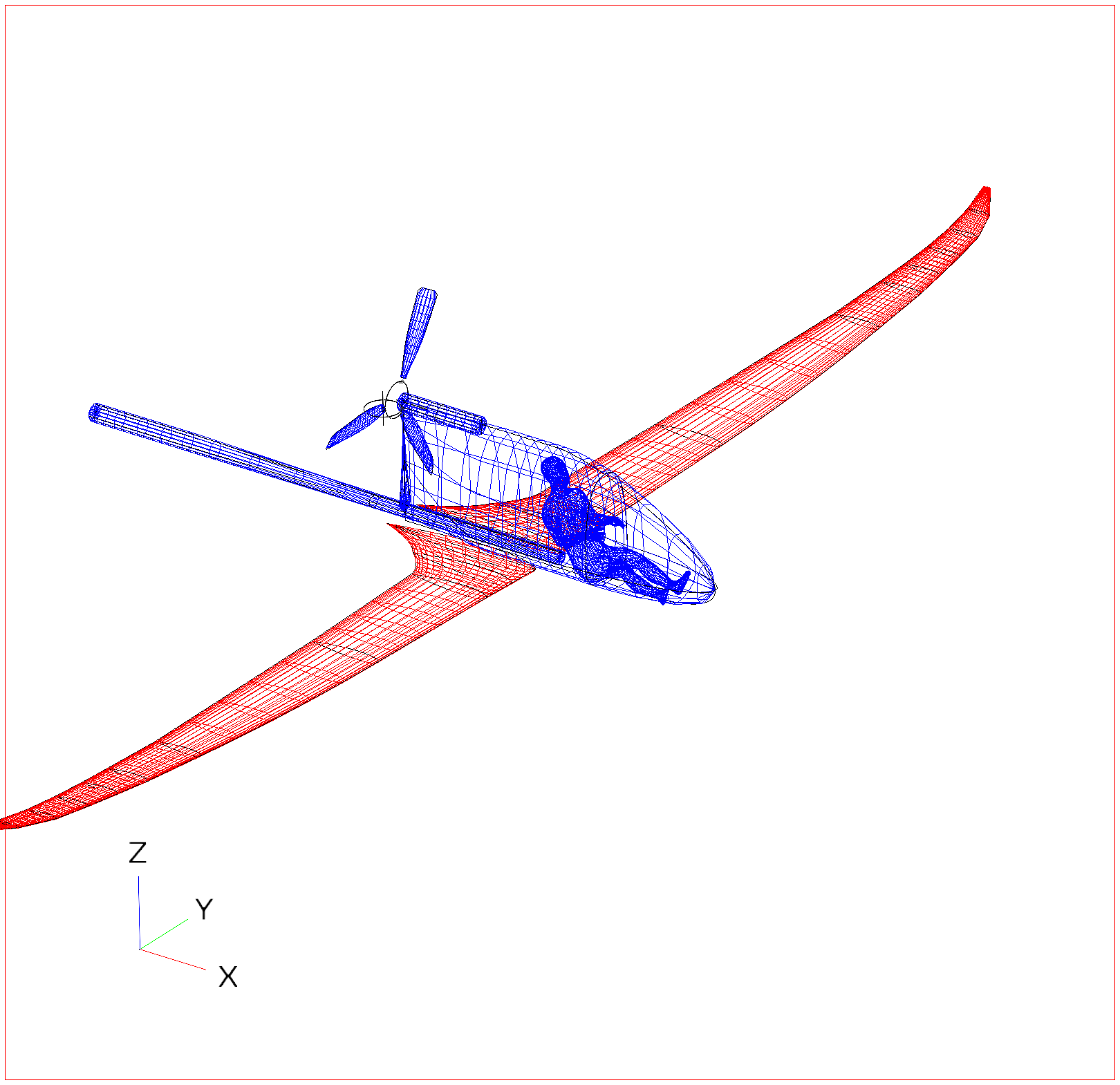
h = 0.03973099856866152
Right, now let’s experiment with three different ways to explore the solution space we created: hill climb, simulated annealing and a genetic algorithm.
Hill Climb
Starting with a similar system to what we used to minimize the fuselage’s cross-sectional area, we can see if we can minimize drag by slowly improving the airplanes frame using feedback from our simulation. For this, we will have to observe every nearby possible state, analyze it, and pick the best of them all. This will guarantee that we will find a minimum/maximum in our solution space. And if your solution space only has one minimum/maximum point, we are guaranteed to find THE best solution. Think of it like trying to climb a pyramid while blindfolded. If there is a stone next to you that is higher than the one you are on, you move to that stone. If there are none, then you are at the top. The algorithm for this is almost as easy as it sounds:
# find and benchmark all neighboring states
for i in range(3, len(sections)):
      pass
      for element in sections[i]:
          pass
          # if 'Angle' in element and 'Top' in element:
          if 'Angle' in element or 'Strength' in element or 'Slew' in element:
              pass
              child = Node(model, i, element, (1 + c), child_number, children)
              child.start()
              child.append(child)
              child_number += 1

              child = Node(model, i, element, (1 - c), child_number, children)
              child.start()
              child.append(child)
              child_number += 1

# set the best one as the parent
for child in children[:]:
      if child.h < parent.h:
          parent = child
Now we press play and watch it take its sweet sweet time until we kill the process and go curse the world for a bit. You see, loading each file, making a change, saving it and running a simulation for 480 states takes too long. I couldn’t go more than 1 iteration in less than 1h (imagine 100 of them). We should’ve thought this out before starting it. The problem has to do with the OpenVSP api not supporting multiple instances on the same process. This means, that we can only open modify and test one model each time. That’s a bummer… but there is a questionable workaround. Python supports multiprocessing with the multiprocessing library. We can create a job for each state we want to explore, and set it loose as a subprocess. This will allow us to benchmark all 480 states in parallel (not exactly all at once, but some). First we’re going to add a function to run the open-modify-heuristic tasks:
def detached_worker(model, i, element, c, child_number, children):
    pass
    value = model['FuselageBase']['XSec'][i][element]['value'] * c
    id = model['FuselageBase']['XSec'][i][element]['_id']
    # create new node
    child = Node(child_number=child_number + 1, model=model)
    child.set_model_param(id=id, value=value)
    # sometimes we get h = 0 becaumax_workers = 4 # max number of subproccesses allowedse of who knows
    children.append(child)
Then we’re going to set a constant that tells the algorithm how many of these workers it can have in parallel (if we have all 480 states running in parallel, we’re going to die), and we’ll add some system to wait for all workers to finish once the number of active workers reaches that threshold:
max_workers = 4 # my number of processors

'''
Inside the loop
'''
  manager = multiprocessing.Manager()
  parent.load_model()
  model = parent.get_model()
  sections = model['FuselageBase']['XSec']
  jobs = []
  child_number = 0
  children = manager.list()

  for i in range(3, len(sections)):
      pass
      for element in sections[i]:
          pass
          # if 'Angle' in element and 'Top' in element:
          if 'Angle' in element or 'Strength' in element or 'Slew' in element:
              pass
              child = multiprocessing.Process(target=detached_worker, args=(model, i, element, (1 + c), child_number, children, ))
              child.start()
              jobs.append(child)
              child_number += 1

              child = multiprocessing.Process(target=detached_worker, args=(model, i, element, (1 - c), child_number, children, ))
              child.start()
              jobs.append(child)
              child_number += 1

          if len(jobs) >= max_workers:
              print('waiting for children...')
              for child in jobs:
                  pass
                  child.join()
              jobs = []

  pool = multiprocessing.Pool(processes=child_number)
  # children = pool.map(child, [c for c in range(child_number)])
  print('done')
  pool.close()
I set the maximum number of workers to 4, because I have 4 cores in my processor. This should (in theory) decrease the time required to run the algorithm by 4. Now we can let the script run for a few hours, and see the results:
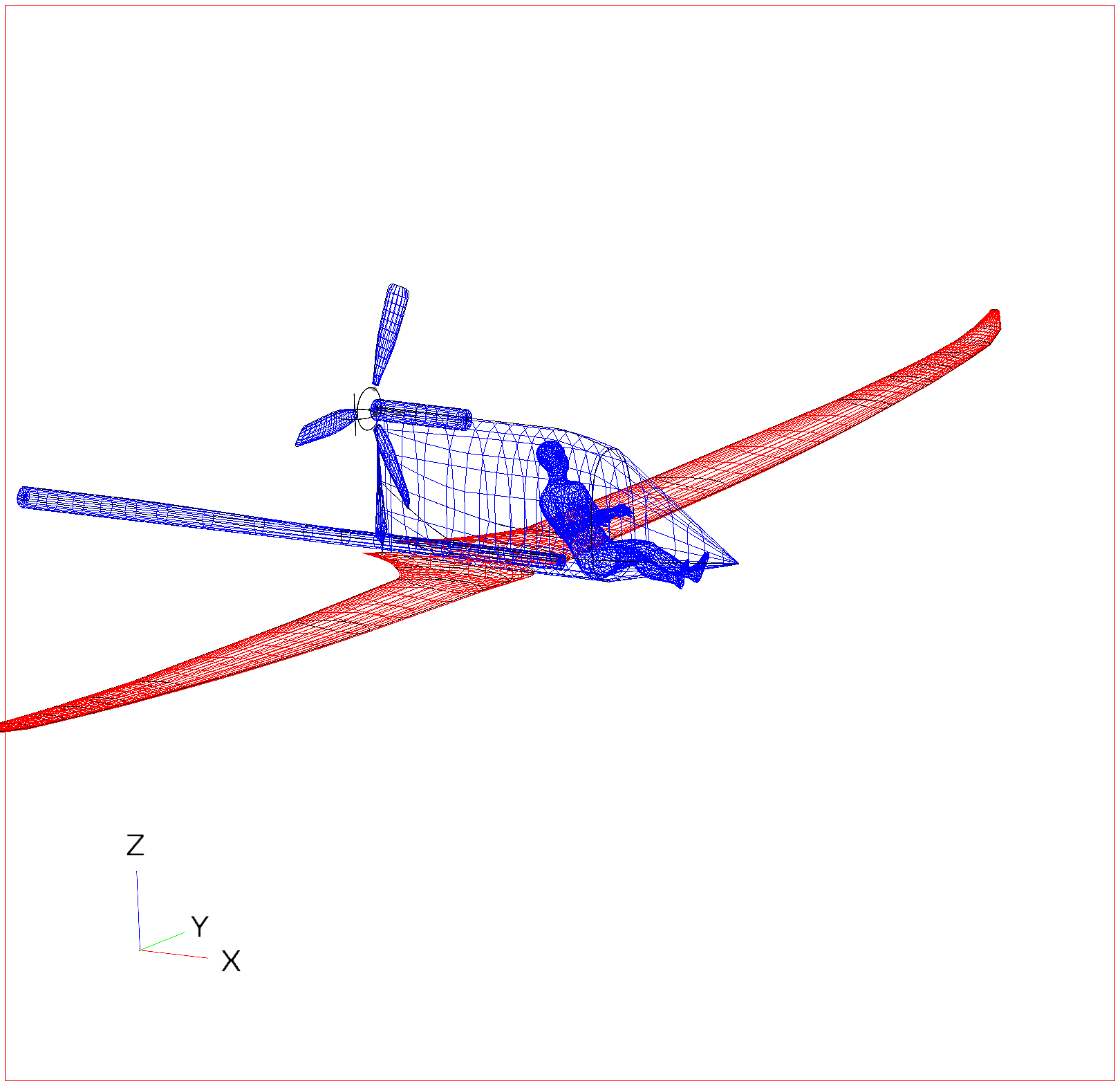
h = 0.03804125029369643
Pointy it is then… I’ve never seen a fuselage like that in my life. Maybe you have, but we can safely agree that it looks odd. This might have something to do with our algorithm choice. Hill climb assumes that there is one only best solution in the entire solution space. But what if there is more than one? What if there are multiple good solutions, but one that is better than the others? Imagine you are blind, and you climbed a pyramid in a field of pyramids. How can you tell that you are on the tallest one? And if you didn’t climb it yet, how can you tell which is going to be the tallest without brute forcing your way up every pyramid? Let’s look at another algorithm.
Simulated Annealing
This strategy is very similar to hill climb, except it has one interesting twist: we add some random “bad” moves to the decision making process. We begin by making almost every move a “bad move” in the beginning, and slowly transition to only “good moves”. If you’ve played guitar before, you know how painful it is to drop your guitar pick inside the the guitar. Removing it is a very complicated process, which resembles this algorithm. You start by shaking your guitar around wildly. You can hear the pick jumping randomly inside the guitar. Eventually, you begin to throw a few subtle swings as an attempt to send the pick closer to the opening. Once it gets close, you become extra careful and calculate every little movement, so you can get the pick out. We’re going to do the same. Let’s start by adding a couple of constants to our code:
import random

def random_step_check():
    global r
    global dr
    return random.uniform(0, 1) < r

...

r = 0.9      # probability of making a wrong step
dr = 0.8      # rate of change of randomness probability
Now, we make use of these in our decision making process:
for child in children[:]:
      if child.h < parent.h or random_step_check():
          parent = child

...

r *= dr
What is happening here is the following: r defines the probability of the next step being made regardless of the heuristic value. In the first iteration, this value is quite high, we will end up picking almost any step. But the probability of making such a move decreases by a factor of dr at the end of each iteration, making it more and more likely that only the best next step be picked. This is what the results look like:
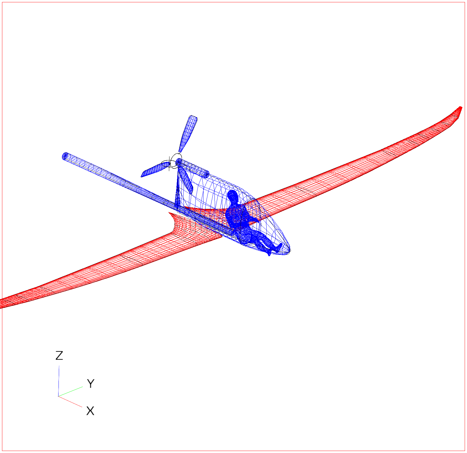
h = 0.0396759160149569
Not so pointy this time. In fact, the result resembles modern gliders a bit more. The final drag coefficient value is slightly larger than the hill climb result.
Evolutionary Progression
Now let’s try something a little different. Genetic algorithms have been around for a while, and they’ve proven to be advantageous when dealing with extremely large solution spaces (such as the one we are dealing with now). I won’t spend much time explaining how a genetic algorithm works; this example does a really good job at it (as long as you’re patient enough to see the results). The code for this is going to look a little different. We are going to start with a population of 10 states, each with one random modification only, generated off of the slimmed down fuselage. We’re generate 100 permutations off of these 10 states with one random modification each. We then benchmark these and pick the 10 best. Rinse and repeat. We can then run this for many many many generations and see what happens. But before, let’s look at the code. We start with the same Node object that we did with the other algorithms, but we’ll change some functions. In order to keep track of every mutation done, we’ll add a list of mutations: self._mutations = [] in the constructor. Then we write the following functions:
def set_model_param(self, id, value):
      pass
      self._model.set_param(id=id, value=value)
      self.save_model()
      self.load_model()
      self.h = self._model.h()
      print('->', self.h)
      self._mutations.append({'id': id, 'value': value})

def set_model_params(self, params):
    pass
    for mutation in params:
        pass
        self._model.set_param(id=mutation['id'], value=mutation['value'])
        self._mutations.append({'id': mutation['id'], 'value': mutation['value']})

    self.save_model()
    self.load_model()
    self.h = self._model.h()
    print('->', self.h)
Then we will modify the function that creates/modifies/benchmarks new nodes:
def detached_worker(mother, father, m, c, child_number, population):
    pass
    global section_start_bound
    model = 0
    # get model
    if mother is not None:
        model = mother.get_model()
    elif model is not None:
        model = m

    # append fathers attributes
    if father is not None:
        mutations = father.get_mutations()
    else:
        mutations = []

    # pick a random attribute
    sections = model['FuselageBase']['XSec']
    elements = sections[random.randint(section_start_bound, len(sections)-1)]
    filtered_elements = list(filter(lambda x: 'Angle' in x or 'Slew' in x or 'Strength' in x, elements))
    random_element = filtered_elements[random.randint(0, len(filtered_elements)-1)]

    # cause a random mutation to the random attribute
    value = elements[random_element]['value'] * (c + 1) * random.uniform(0, 1)
    id = elements[random_element]['_id']
    mutations.append({'id': id, 'value': value})

    # give birth
    child = Node(child_number=child_number + 1, model=model)

    # set parameters
    child.set_model_params(mutations)

    # sometimes we get h = 0 because of who knows
    population.append(child)
Notice it now receives two parents or a model, creates a child based on the mother, applies the mutations of the father if they exist, makes a random mutation, benchmarks the child, and adds it to the population list. Next, before our routine we need a way to start a parent population:
# start population
for i in range(0, int(population_size/10)):
    parent = Node(starting_model, filename=filename)
    parent.h = 99
    child = multiprocessing.Process(target=detached_worker, args=(None, None, starting_model, c, child_number, parent_population, ))
    child.start()
    jobs.append(child)
    parent_population.append(parent)
Note that we are passing the starting_model instead of passing it parents, because there are no parents. Also notice how the parent population size is 10% that of the child population size. Then, in our routine, we need to create the parent’s offspring as such:
for mother in parent_population:
      for father in parent_population:
          pass
          child = multiprocessing.Process(target=detached_worker, args=(mother, father, None, c, child_number, population, ))
          child.start()
          jobs.append(child)
          child_number += 1
For each parent, we will create a child with each other parent. This does mean that each parent will have a child with itself, so technically the species is parthenogenic. Finally, we need to pick the next generation of parents once the child population has been benchmarked:
parent_population = sorted(population[:],key = lambda x: x.h)[:len(parent_population)]
And then pick the best parent of the lot once the routine is complete:
winner = parent_population[0]
Is easy. Let’s look at the results after 100 generations of 100 children and 10 parents each:
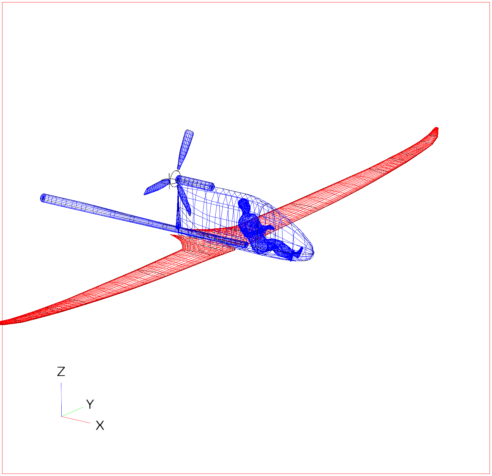
h = 0.03824597600673088
Better than Simulated Annealing, but worse than Hill Climb. And it looks quite similar to the starting model.
The Best Way To Make Money In Mount And Blade 2: Bannerlord
While we wait for these algorithms to finish their job, let’s play some of that Bannerlord goodness I’ve been waiting for since 2012. I like to play as a rogue horse archer that doesn’t get too much into politics, but still makes money. First I’m going to visit as many cities as possible, to get an idea of what prices are being asked around. Next, I will find a village that produces some sort of good, such as ores or grain. When hovering over the prices of goods, if the price is green, I buy them in bulk. Then I travel to some city where the villages around do not produce this good I just bought. This will yield a better profit. If the price of the goods I want to sell are red, I sell them in bulk. It should take a couple of in game weeks to reach a 4k-5k. Now it’s time for serious cash: horse trading. There are breeds of horses that are specific to certain parts of the world, that sell for a lot in other parts of the world. Specifically, Aserai horses. They can be bought in towns in the desert for less than 1.2k, and can be sold for upwards of 2k in colder climates. The nice thing about trading horses, is that they don’t really add any weight to your inventory so you can carry as many as you’d like. Plus, you can stock up on other goods (such as dates) thanks to the extra carrying capacity horses provide. Doing this a couple of times can provide enough income to invest in a passive income source (where you don’t need to do anything). I bought a pottery studio in a town surrounded by towns that provide clay. This yields about 200 per day, which is largely enough for me to roam the world with my 3 companions. But it doesn’t stop there if you want to make money. The income generated by workshops depends on the price of goods in the local city’s marketplace. Pottery is made from clay. If we manage to flood the market with clay, the price of clay will go down. We can also buy all the pottery at a cheap price (the workshop will flood the market with pottery), and sell it to other cities. This will maximize our profit margins to upwards of 300 per day, plus the profit generated by selling the pottery around the world. I’ve only been playing for 2 (real) days, so I haven’t had the chance to experiment with other options, but here’s what I’m going to experiment with next: as a workshop becomes productive, its resale value increases. My thoughts are, that if I can get my pottery studio to make a lot of revenue, I can flip it for a lot of money, force it to lose value by buying all of the clay supply, and but the workshop again at a low price. Maybe next week we’ll know if that works.
What Could Be Done Better
Let’s talk about the size of the solution space. Watching the changes being done by the algorithm, one can notice that not all changes affect the heuristic value or the design at all. Also, playing with the OpenVSP editor, I could not find a way to create a shape using the Slew property, that I could not reproduce using the Strength property. Furthermore, assuming symmetry to be part of the ultimate solution might not be a bad shortcut; there are only a handful of asymmetrical airplane designs out there, and most aren’t what you would call optimal (although they do look quite appealing). It might not be worthwhile to investigate these items, because we already have a decent fuselage design. But the wings and the tails will come next, and that will be a real challenge for our slow-and-resource-hungry-as-hell algorithms. When it comes to the algorithms, systems could be used to decrease their time complexity a bit. Hill Climb will go on until the time is over, constantly making smaller and smaller changes. To make the algorithm more deterministic (and potentially faster) it would be a smart idea to make it stop once it finds a state that happens to be better than all its neighbors. Simulated Annealing could probably benefit from a change of routine. Instead of picking a random state from the list of neighboring states, it would be a lot faster to determine if it will pick a random state before discovering all the neighbors. Then it can pick a random state, without even running the heuristic. This could dramatically increase performance, and solution space covered. As for the evolutionary progression, studying the right amount of random mutations could be beneficial. Here’s why: with each generation, the children are an agglomerate of the parent’s mutations, with one random mutation. They are not too far from the definition of a permutation. This leads to a very slow solution space exploration. Perhaps a more efficient routine would consist of mostly random mutations in the beginning, but more permutations close to the end.
Thanks!
See my previous and my next post 🙂
-by Eduardo”